


- Introduction
- The Problem
- Solution
- Setup
- Running a pre-trained Detectron2 model
- Image manipulation with Python
- Final Thoughts
TL;DR
The goal of this tutorial is to describe one method of automating the process of cutting out objects (things, people, pets, etc.) from images and combining them to make a collage of sorts.
First, I go through creating binary masks for one or more objects in an image by using a class of computer vision algorithms called image segmentation. Binary mask(s) in hand(s), I go through one method (technically two, actually) of using said binary mask(s) to extract or remove part(s) of an image. Next, I do some basic image transformations (rotate, crop, and scale) on the resulting cutout. Finally, I paste the cutout on top of another image to make a collage.
Rather than drawing binary masks by hand or using proprietary software like Photoshop to manipulate and transform images, I'll show you how to automate the process using completely free, open-source tools. Namely, we'll be using Python along with a few open-source libraries:
The Problem
Selecting and separating parts of an image can be a tedious, time-consuming process. Anyone who's done a fair amount of tinkering with image manipulation using a program like Photoshop knows the struggle.
Although modern tools make the process easier, wouldn't it be nice if there was a way to automate the process?
Creating "Paws"
As an example, say I'd like to cut out my cat Hobbes from a photo in order to "Photoshop" him into a different image. Here's the photo of Hobbes I'll be using.
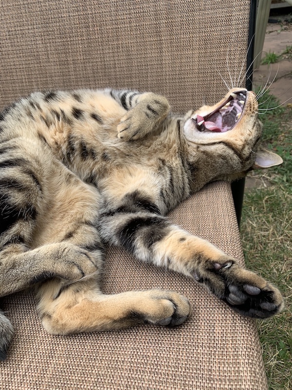
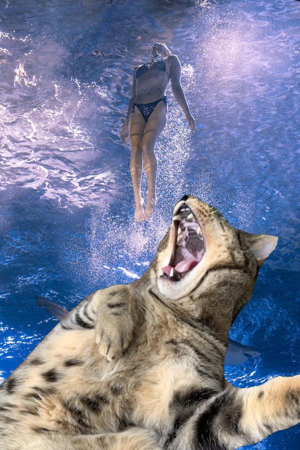
I think his position is perfect for creating "Hawbbes" (Jaws + Hobbes)...meh I'll call it "Paws". By cutting him out and rotating him a bit, he could be pasted onto an underwater shot of someone swimming and he could live his dream of being a fierce sharkitty.
Here's an image I found on Unsplash that would work as the background onto which Hobbes, once cut out of the image above, can be pasted.
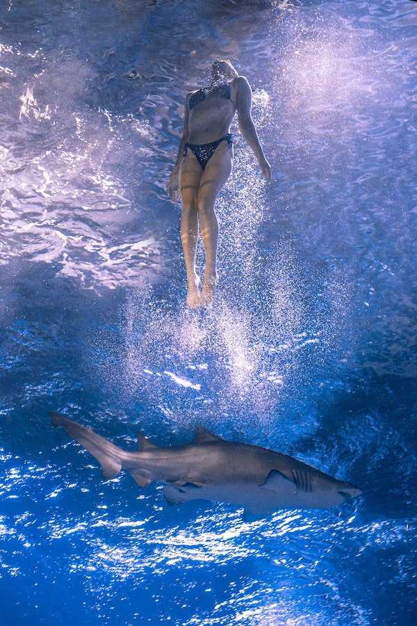
Basically, in order to cut Hobbes out of the photo above, I'll have to make all the pixels in the image transparent except for the ones representing Hobbes. Then I'll crop, rotate, scale, and superimpose the resulting image on top of the underwater shot such that Hobbes roughly takes up the bottom half.
Image Masking
To accomplish this manually, I could spend anywhere from a few minutes to a few hours outlining Hobbes in the original image to create a mask — masking the image. The time investment depends on how easily-separable the subject is from the rest of the image, how accurate I want the cut to be, and what tools are available to me.
Regarding that last point, the magicians at Adobe have done some rather impressive black magic with Photoshop, giving users very quick and very effective methods for selecting parts of an image. However, the goal of this post is to accomplish this programmatically, without the use of any closed-source software.
A mask is basically a method of distinguishing/selecting/separating pixels. If you've never heard the term used this way before, one way to think about it is with masking tape and paint. Typically, one would put masking tape—i.e. create a "mask"—around areas on a wall that should not be painted. This is essentially what a mask is doing in any photo manipulation software: indicating what areas of an image to affect or transform (or which areas not to do so).
Here's the image of Hobbes with the image segmentation-generated masks overlayed on top of it (which we'll be creating later) showing, obviously, where Hobbes is in the image. It doesn't really matter that the model thinks he's a dog — we won't be using the predicted class, only the mask. And the mask is still good enough for our purposes.
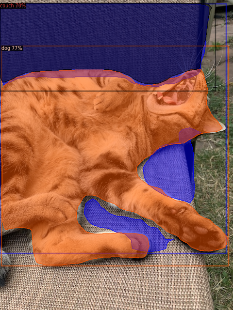
A binary mask is a method of masking which uses a two-tone color scheme, to indicate the areas of an image to be affected and not affected. By overlaying a binary mask on top of the original image, the boundaries between the two colors can be used to affect the different areas of the image differently, whether that is making pixels transparent (removing them) or applying some sort of effect or transformation.
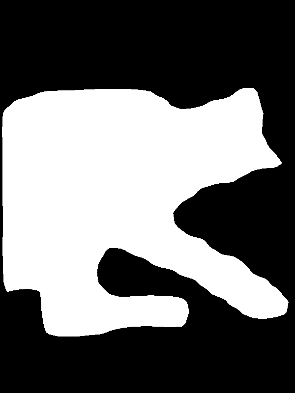
The white area in the image below shows the same coordinates as the orange one above, converted into a binary mask. While I've only spent any significant time with Photoshop, I'd imagine any decent image manipulation software can work with binary masks similarly to how we'll be working with them.
Computer vision
In order to generate binary masks based on the content of the image, the algorithm must be somewhat intelligent. That is, it must be able to process the image in such a way that it can recognize where the foreground is and draw a polygon around it with some degree of accuracy.
Luckily, there are a number of deep learning models that will do just that. The field is called Computer Vision, and the class of algorithm used in this article is known as image segmentation.
Don't worry if you don't have any experience with this type of thing, or even if you don't necessarily want to get experience with it. Modern machine learning tooling makes it incredibly quick and easy to get a model up and predicting with pre-trained weights. Though if you want to understand what's going on, it will likely help to know a bit of Python programming.
One caveat: the pre-trained models will usually work well with classes of objects that were in their training data. The model weights used in this post were trained on the COCO dataset, which contains 80 object classes. Depending on what the object in the foreground is that you are trying to extract, you may or may not need to extend the model with a custom dataset and training session. That is a topic for another post.
Detectron2
The deep learning framework used here is PyTorch, developed by Facebook AI Research (FAIR). More specifically, we'll use a computer vision framework, also developed by FAIR, called Detectron2.
Although the primary framework used in this article is Detectron2, this process should be translatable to other image segmentation models as well. In fact, I'll be adding an addendum to this post in which I'll go over using Matterport's TensorFlow-based implementation of Mask R-CNN to accomplish the exact same thing.
Heck, while I'm at it, I might as well do it with fastai as well.
Setup
Install Detectron2 and other dependencies
As mentioned in the introduction, the framework we'll be using for image segmentation is called Detectron2. The following cells install and set up Detectron2 in a Google Colab environment (pulled from the official Detectron2 getting started notebook). If you don't want to use Colab for whatever reason, either play around with installation and setup or refer to the installation instructions.
The other top-level dependencies needed for this tutorial:
The nice thing about Colab is all of these come pre-installed. Oh yeah, you also get free access to a GPU. Thanks, Googs!
Again, simply click the "Open in Colab" badge at the top of this page, then hit File > Save a copy in Drive, which does exactly what it says: saves a copy of the notebook to your Google Drive. In addition, you can open an ephemeral copy of the notebook without saving it first by hitting File > Open in playground mode.
Once you have everything installed, we can start with some imports and configuration.
# === Some imports and setup === #
# Setup Detectron2 logger
import detectron2
from detectron2.utils.logger import setup_logger
setup_logger()
# Common libraries
import numpy as np
import os, json, cv2, random
# Only needed when running in Colab
from google.colab.patches import cv2_imshow
# Detectron2 utilities
from detectron2 import model_zoo
from detectron2.engine import DefaultPredictor
from detectron2.config import get_cfg
from detectron2.utils.visualizer import Visualizer
from detectron2.data import MetadataCatalog, DatasetCatalog
Most, if not all, open-source deep learning frameworks have a set of pre-trained weights available to use. The creators of the frameworks will conduct a series of training sessions on the most commonly-used datasets in order to benchmark the performance of their algorithms. Luckily for everyone else, they typically provide the results of this training in the form of weights, which can be loaded into the model and be used for inference immediately.
For many tasks, including recognizing and outlining an image of a cat, pre-trained weights will work fine. The model weights used in this post were trained on the popular COCO dataset, which contains 80 object classes, including cats. If, for example, we wanted to do the same thing with whales or one specific person, we'd have to do some custom training.
I will be publishing a companion blog post to this one about training Detectron2 on a custom dataset. Once that is published, I'll link to it here. If there's no link yet, I haven't published it yet.
If you're curious about custom training now, the Detectron2 "Getting Started" Colab notebook also goes through one way of doing so.
!wget https://raw.githubusercontent.com/tobias-fyi/assetstash/master/visual/images/img_seg_bin_mask/01_hobbes.jpg
im = cv2.imread("./01_hobbes.jpg")
If you think about what a digital image actually is, it makes sense to represent it as a matrix — each row corresponds to a row of pixels, and each column a column of pixels in the image. Technically, images would be considered a 3-dimensional array, because they have width, height, and depth (number of channels).
Depending on if the image has three channels (typically RGB: red, green, blue) or four (typically RGBA: same plus an alpha channel), the values at each row-column index (or cell, like in a spreadsheet, in case that helps you visualize it) indicate the intensities of each of the color channels (and transparency, in the case of 4-channel images) for each pixel.
Thus, after the image is loaded, it really is just an array of numbers and can be utilized and manipulated just like any other array. For example, in order to rotate the image, a linear transformation can be applied to the image matrix to "rotate" the pixel values within the matrix.
Here is an example of a single row in the array representing the image of Hobbes is shown.
# === Look at the image, in array form === #
print("Image dimensions:", im.shape)
print("\nImage array - first row of 3-value sub-arrays:")
im[0]
# === Look at the image, rendered === #
cv2_imshow(im)

Inference with Detectron2
After the image is loaded, we're ready to use Detectron2 to run inference on the image and find the mask of Hobbes. Running inference means generating predictions from the model. In the case of image segmentation, the model is making a prediction for each pixel, providing its best guess at what class of object each one belongs to, if any.
We create a Detectron2 config and instantiate a DefaultPredictor, which is then used to run inference.
Just a heads-up: the first time this runs, it will automatically attempt to start downloading the pre-trained weights — a ~180mb pickle file. That's a lot of pickles...
In addition to downloading and configuring the weights, the threshold is set for the minimum predicted probability. In other words, the model will only output a prediction if it is certain enough — the probability assigned to the prediction is above the threshold.
# Add project-specific config (e.g., TensorMask) here if you're
# not running a model in Detectron2's core library
cfg = get_cfg()
cfg.merge_from_file(model_zoo.get_config_file("COCO-InstanceSegmentation/mask_rcnn_R_50_FPN_3x.yaml"))
cfg.MODEL.ROI_HEADS.SCORE_THRESH_TEST = 0.5 # set threshold for this model
# Find a model from detectron2's model zoo. You can use the https://dl.fbaipublicfiles... url as well
cfg.MODEL.WEIGHTS = model_zoo.get_checkpoint_url("COCO-InstanceSegmentation/mask_rcnn_R_50_FPN_3x.yaml")
predictor = DefaultPredictor(cfg)
outputs = predictor(im)
By default, the output of the model contains a number of results, including the predicted classes, coordinates for the bounding boxes (object detection), and mask arrays (image segmentation), along with various others, such as pose estimation (for people). More information on the types of predictions made by Detectron2 can be found in the documentation.
We are really only interested in the one mask outlining Mr. Hobbes here, though will also need to extract the IDs for the predicted classes in order to select the correct mask. If the image only has one type of object, then this part isn't really necessary. But when there are many different classes in a single image, it's important to be certain which object we are extracting.
First, let's take a look at how the model did.
v = Visualizer(im[:, :, ::-1], MetadataCatalog.get(cfg.DATASETS.TRAIN[0]), scale=0.8)
out = v.draw_instance_predictions(outputs["instances"].to("cpu"))
cv2_imshow(out.get_image()[:, :, ::-1])

Extracting the mask
The "dog" is the first id in the .pred_classes list. Therefore, the mask that we want is the first one in the .pred_masks tensor (array).
Those colored areas are the "masks", which can be extracted from the output of the model and used to manipulate the image in neat ways. First, we'll need to get the array holding the mask.
In this case, as can be seen below, each mask is a 2-dimensional array of Boolean values, each one representing a pixel. If a pixel has a "True" value, that means it is inside the mask, and vice-versa.
print(outputs["instances"].pred_classes)
print(outputs["instances"].pred_masks)
# List of all classes in training dataset (COCO)
# predictor.metadata.as_dict()["thing_classes"]
# The class we are interested in
predictor.metadata.as_dict()["thing_classes"][16]
# Find the index of the class we are interested in
# First, convert to numpy array to allow direct indexing
class_ids = np.array(outputs["instances"].pred_classes.cpu())
class_index = np.where(class_ids == 16) # Find index where class ID is 16
# Use that index to index the array of masks and boxes
mask_tensor = outputs["instances"].pred_masks[class_index]
print(mask_tensor.shape)
mask_tensor
hobbes_mask = mask_tensor.cpu()
print("Before:", type(hobbes_mask))
print(hobbes_mask.shape)
hobbes_mask = np.array(hobbes_mask[0])
print("After:", type(hobbes_mask))
print(hobbes_mask.shape)
hobbes_mask
# The "True" pixels will be converted to white and copied onto the black background
background = np.zeros(hobbes_mask.shape)
background.shape
bin_mask = np.where(hobbes_mask, 255, background).astype(np.uint8)
print(bin_mask.shape)
bin_mask
cv2_imshow(bin_mask)

Using the binary mask to cut out Hobbes
In order to use numpy operations between the mask and image, the dimensions of the mask must match the image. The image array has three values for each pixel, indicating the values of red, green, and blue (RGB) that the pixel should render. Therefore, the mask must also have three values for each pixel. To do this, I used a NumPy method called np.stack to basically "stack" three of the masks on top of one another.
Once the dimensions match, another NumPy method, np.where, can be used to copy or extract only the pixels contained within the area of the mask. I created a blank background onto which those pixels are copied.
# Split into RGB (technically BGR in OpenCV) channels
b, g, r = cv2.split(im.astype("uint8"))
# Create alpha channel array of ones
# Then multiply by 255 to get the max transparency value
a = np.ones(hobbes_mask.shape, dtype="uint8") * 255
print(b.shape, g.shape, r.shape, a.shape)
# We want the image to be fully opaque at this point
a
# Rejoin with alpha channel that's always 1, or non-transparent
rgba = [b, g, r, a]
# Both of the lines below accomplish the same thing
im_4ch = cv2.merge(rgba, 4)
# im_4ch = np.stack([b, g, r, a], axis=2)
print(im_4ch.shape)
cv2_imshow(im_4ch)

# Create 4-channel blank background
bg = np.zeros(im_4ch.shape)
print("BG shape:", bg.shape)
# Create 4-channel mask
mask = np.stack([hobbes_mask, hobbes_mask, hobbes_mask, hobbes_mask], axis=2)
print("Mask shape:", mask.shape)
# Copy color pixels from the original color image where mask is set
foreground = np.where(mask, im_4ch, bg).astype(np.uint8)
# Check out the result
cv2_imshow(foreground)

The Roundabout Method
This is that "second" method I talked about in the introduction.
This is how I added a fourth channel to the image after the fact, once the colored pixels had been copied onto a black background. While this method works, I'm sure you can think of one primary issue with it.
It took me too long to realize this, but by using a black background and the method below, which converts all black pixels to transparent, any pixels brought over from the original image that also happened to be black were converted to transparent.
That's why I decided to refactor into the method above.
However, I felt like I should leave it in anyways, as it still has some potentially useful code in it. For example, in the case when the image cannot be converted to four channels beforehand.
bg = np.zeros(im.shape)
bg.shape
mask = np.stack([hobbes_mask, hobbes_mask, hobbes_mask], axis=2)
foreground = np.where(mask, im, bg).astype(np.uint8)
# i.e. add the alpha channel and convert black pixels to alpha
tmp = cv2.cvtColor(foreground.astype("uint8"), cv2.COLOR_BGR2GRAY)
_, alpha = cv2.threshold(tmp, 0, 255, cv2.THRESH_BINARY)
b, g, r = cv2.split(foreground.astype("uint8"))
rgba = [b, g, r, alpha]
dst2 = cv2.merge(rgba, 4)
# Look at the result, if needed
# cv2_imshow(dst2)
Image manipulation with Python
Now, this image can be saved (as a PNG to preserve the alpha channel/transparency) and simply overlayed onto another image. Or, even better, the image can be used directly (as it is now, in the form of an array), scaled, rotated, moved, then pasted overtop of the other image.
At first I was going to use Photoshop to overlay Hobbes and make him look like a super dangerous sharkitty. But then I remembered the goal of this post, and decided to do it programmatically with Python.
The primary library I'll be using to manipulate images is Pillow.
from PIL import Image
# Use plt to display images
import matplotlib.pyplot as plt
%matplotlib inline
!wget https://raw.githubusercontent.com/tobias-fyi/assetstash/master/visual/images/img_seg_bin_mask/05_jaws_kinda.jpg -q -O 05_jaws_kinda.jpg
jaws_img = Image.open("05_jaws_kinda.jpg")
# Dimensions of background image (600, 900) will be useful later
print(jaws_img.size)
plt.imshow(jaws_img)

# Found here: https://stackoverflow.com/a/9042907/10589271
# There is another (potentially easier) way to do it with Pillow, using Image.rotate()
def rotate_image(image, angle):
image_center = tuple(np.array(image.shape[1::-1]) / 2)
rot_mat = cv2.getRotationMatrix2D(image_center, angle, 1.0)
result = cv2.warpAffine(image, rot_mat, image.shape[1::-1], flags=cv2.INTER_LINEAR)
return result
fg_rotated = rotate_image(foreground, 45)
cv2_imshow(fg_rotated)

Load into Pillow
Once the image is rotated, it needs to be cropped and scaled appropriately. I decided to use Pillow for these transformations. For some reason that I have not looked into yet, OpenCV images are in BGR (blue, green, red) format instead of the virtually universal RGB format. Thus, in order to load the image from cv2 into Pillow without reversing the blues and reds, the color first must be converted to RGB.
Once converted, it can simply be loaded into Pillow as a PIL.Image object, which contains a suite of useful methods for transformation and more.
# Convert color from BGRA to RGBA
fg_rotated_fixed = cv2.cvtColor(fg_rotated, cv2.COLOR_BGRA2RGBA)
# Load into PIL.Image from array in memory
hobbes_rotated = Image.fromarray(fg_rotated_fixed)
plt.imshow(hobbes_rotated)

Crop
I manually defined the coordinates of the box used to crop the image by eyeballing it (shout out to Matplotlib for including tick marks on rendered images). A more automated method for doing this would be to extract the bounding box coordinates from the model output, and use that to crop the image before doing any other transformations. I will add this to a later iteration of this tutorial (if you're reading this, it likely hasn't been implemented yet).
box = (0, 80, 480, 500)
crop = hobbes_rotated.crop(box2)
print(crop.size)
plt.imshow(crop)

Resize
Next, the cropped and rotated image must be resized in order to fill up the entire width of the background onto which it will be pasted. The reason for this is simply because the dimensions of the "paste" box must exactly match that of the "copy" box. It must be explicit — i.e. it's not like Photoshop where any of the image falling outside the boundaries of the "canvas" is cropped or simply left out.
width = jaws_img.size[0]
scale = width / crop.size[0] # Calculate scale to match width
height = int(scale * crop.size[1]) # Scale up height accordingly
new_size = (width, height)
# Resize!
resized = crop.resize(new_size)
print(resized.size)
plt.imshow(resized)

paws = jaws_img.copy()
# Paste box dimensions have to exactly match the image being pasted
paste_box = (0, paws.size[1] - resized.size[1], paws.size[0], paws.size[1])
paws.paste(resized, paste_box, mask=resized)
plt.imshow(paws)

paws.save("06_paws.jpg")
Potential improvements
As with just about any process, there are always aspects that could be changed in an effort to improve efficiency or ease-of-use. I will keep adding to this list of potential improvements as I think or hear of them:
- Fully automated the crop by using the bounding box from the model output
Further Work
There are a couple of additional adjacent projects to this that I'd like to work on at some point in the future, both to help others use the method outlined above, and to give me practice with various other aspects of the development lifecycle.
The two projects I have in mind are essentially the same thing, accomplished different ways. First, I'd like to integrate this method into a Python package and put it on PyPI so it can be installed with Pip and easily customized/used from the command line or in other scripts. Second, I want to build a simple web app and API that would allow anyone to upload an image, choose a class of object to extract (or remove), run the model, then download the image with the background (and/or other objects) removed.
As I work on these, I'll put links here.